Parse and plot activity data interactively in Jupyter with GPSbabel, Gpxpy, Geopy and Gmaps

In the last months it seemed that everyone is joining Strava. It may due to that we’re all tired of staying in our homes during the COVID-pandemic. Or it may be due to the fact that almost half of all people have gained weight due to lack of movement. Whatever the reason, Strava has gained a lot of users. However, if you are an OG user and have joined before May 20th, 2020, you’ll know that there were many useful features that are now locked behind the Strava subscription. For example, the leaderboard, matched runs and route builder are all only for those that pay a minimum of around $5 per month. For many, it is just not woth it.

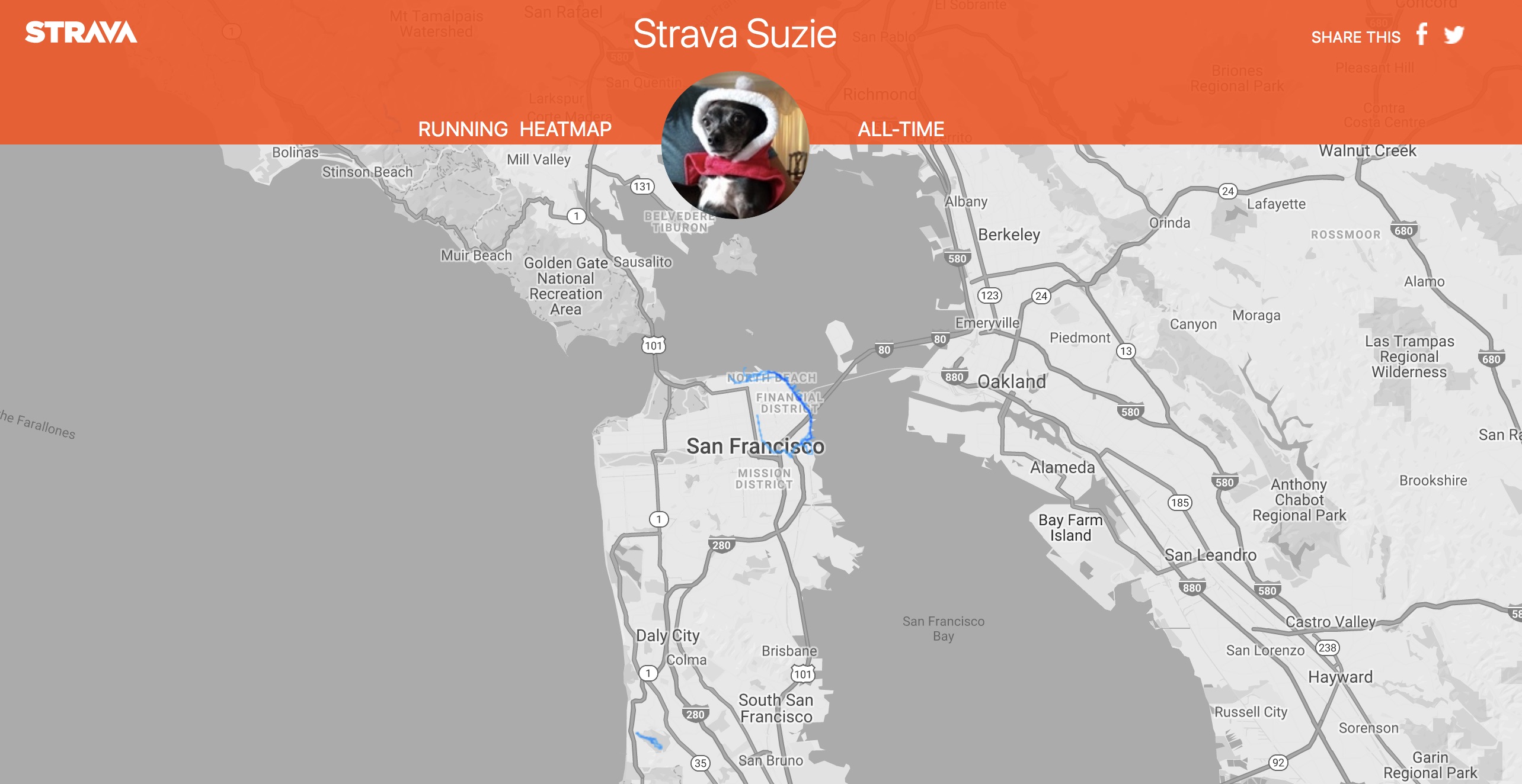
On of the removed features that I really enjoyed was the personal heatmap, on which you’re activities are beautifully plotted on a stylized instance of Google Maps. Maybe it’s just because I’m a sucker for these kind of things, but seeing everywhere I’ve run gave me a sense of accomplishment, as if my runs are engraved into the asphalt and bricks of these roads on the heatmap.

So, why don’t we build our own heatmap from your personal data? And along the way, let us add some more functionality and customization options to really make the heatmap our own. In this implementation, we can selectively show data based on location, time, or any time of metadata, and additional configure the look of the map to any style configured on the Google Maps Platform Styling Wizard. Note that you’ll need a Google Cloud Platform account and a Google Maps API key.

Your Strava data

Your personal data and bulk can be exported from Strava by following this guide. You’ll notice that this is zipped folder containing quite a few files. We are interested in the activities.csv and the activities folder. The csv file is a list of all your activities, and contains metadata such as the activity type, average cadence and calories burned.

The activities folder contains the files associated with every individual activity. The file type for every activity is actually dependent on the device used for tracking, and may either be .gpx or .tcx, a compressed .gz file, or some other filetype that I didn’t come across. I mostly use fitness watch to track my activities, but sometimes use my phone as well. We’ll need to make sure that all filetypes can parsed by our program. I’ve tried many gpx, tcx or general xml parsers. But none seems to be as reliable as GPSbabel. The installation instructions for GPSbabel are here.

Parsing data in Jupyter notebook

There is a Jupyter notebook related to this blog post. Find the notebook here. Within our Jupyter notebook, we first utilize GPSbabel to convert all activities files to a unified gpx format. This can be simplify done using our function parse_activities().

folder = "../EXPORT_########/"
files = parse_activities(folder, folder + "activities", folder + "activities.csv")

Next, we’ll use gpxpy to parse all gpx activities. It might be necessary to install my fork of gpxpy. The instructions are included in the notebook. On my fitness watch, the Amazfit Stratos 2, some trckpts (track-points) in the gpx file do not include longitude and latitudes, to which gpxpy throws an error. It might not be necessary for your devices.

Using gpxpy, we parse all activities into a Pandas dataframe. In this dataframe, each row is a tracked location containing a longitude, latitude and timestamp. We separate the timestamp into columns for easier data selection using Pandas methods. Also, we use GeoPy to find the starting position of each activity. We limit the number of calls to the Geopy to 1 call per second. Change the value for user_agent if necessary.

data = []
locator = Nominatim(user_agent="YOUR_CUSTOM_AGENT").reverse
lim_locator = RateLimiter(locator, min_delay_seconds=1)

for filename, activity_type in prog(files.items()):
    # Parse with gpxpy
    with open(folder + filename, "r") as file:
        gpxdata = gpxpy.parse(file)

    for track in gpxdata.tracks:
        for segment in track.segments:
            # Locate segment starting location
            locdict = lim_locator("{}, {}".format(point.latitude,
                point.longitude), language='en').raw

            # Save segment data to mydict
            mydict = {
                "year"      : point.time.year,
                "month"     : point.time.month,
                "weekday"   : point.time.weekday(),
                "hour"      : point.time.hour
            }
            for key in ["country", "state", "city"]:
                mydict[key] = locdict["address"][key]
                    if key in locdict["address"] else "Unknown"

            for point in segment.points:
                if point.latitude and point.longitude:
                    # Append row with location and all items in mydict
                    data.append(dict(
                        latitude    = point.latitude,
                        longitude   = point.longitude,
                        time        = point.time,
                        type        = activity_type,
                        file        = filename,
                        **mydict
                    ))

df = pd.DataFrame(data)
print("Dataframe ready")

Plotting on top of an interactive Google Maps window

Finally, we plot interactively on Google Maps via gmaps. The documentation is provided here. As mentioned ealier, you’ll need a Google Cloud Platform account and a Google Maps API key. How to acquire this key for yourself can be found in the documentation of gmaps. We configure our PlotApp such that any column in the dataframe can be enabled as a selectable category in the interactive window. See plotter.py for more details

api_key = "AI....."
categories = ["city", "type"]

map = PlotApp(api_key, df, categories)
map.render()

The heatmap gradient can be changed by supplying a list of colors from a list of basic CSS colors or in tuple format for RGB or RGBA.

map.heatmap.gradient = [
    (0,0,0,0),
    'blue',
    'purple',
    'red'
]

If the one wants to customize the style of the background map, we will need to install the version of Gmaps of this pull request. The pull request is fully functional, but development on Gmaps is seemingly inactive. The installation instructions are included in the notebook. A custom map style can be created in the Google Maps Platform Styling Wizard. The outputted JSON is to be saved as a string to the map.fig.styles attribute

Notice that with gmaps, we can change the colors of the heatmap and the background map itself after the map has been rendered. This is great! We can make it look exactly as we like to.

The downside to this application is that dimension of the exported image cannot be specified. The quality of the image is limited to the interactive window.